Beyond the Notebook: Building an End-to-End E-Commerce Analytics API
Moving beyond Untitled.ipynb: A journey of OOP, SQL, and FastAPI.
Introduction: Why I Built This?
Data science learning paths often start and end in Jupyter Notebooks. While notebooks are fantastic for exploration, they rarely represent how machine learning works in the real world.
This project is a medium-scale (i think this is medium-scale) milestone in my development roadmap. My goal was not just to train a model, but to build a sustainable data science system that:
• Stores data efficiently in an SQL database.
• Adheres to Object-Oriented Programming (OOP) principles.
• Optimizes its own ingestion process (Smart ETL).
• Serves predictions to the outside world via a REST API.
In this article, I will walk you through how I built an E-Commerce Analytics system that handles Customer Segmentation, Churn Prediction and CLV (Customer Lifetime Value) forecasting.
Software Architecture
Why not just use a Notebook? Because for a sustainable system, code must be modular, readable, and extensible. I organized the project under a src/ directory, dividing it into classes with clear responsibilities.
The Project Structure:
Ecommerce_Project/<br>
├── artifacts/          # Stores trained models (.pkl)<br>
├── data/               # Raw CSVs and processed data<br>
├── db/                 # SQLite database storage<br>
├── notebooks/          # For initial EDA and experiments<br>
├── src/                # Core Application Logic<br>
│   ├── __init__.py<br>
│   ├── api.py          # FastAPI endpoints<br>
│   ├── config.py       # Centralized configuration<br>
│   ├── data_ingestion.py   # Smart ETL (Hash check)<br>
│   ├── data_processor.py   # Cleaning & Feature Eng.<br>
│   └── model_trainer.py    # Training pipelines<br>
├── main.py             # Orchestration script<br>
└── requirements.txt
Data Persistence (SQLite)
Instead of re-reading a 1,000,000-row CSV file during every execution, I processed the data once and saved it to a SQLite database using SQLAlchemy. This allowed me to proceed much faster in subsequent steps using SQL queries.
The “Smart Ingestion” Trick
One of the features I’m most proud of is the MD5 Hash Check in the DataIngestion class. In previous projects, I wasted time while setting files.
Here, the system calculates a “fingerprint” of the raw CSV file. If the file hasn’t changed, it skips the heavy ingestion and cleaning steps entirely.
# src/data_ingestion.py
def check_for_new_data(self):
    """
    Checks if the CSV file has changed using MD5 Hashing.
    Returns True if changed or first run.
    """
    current_hash = self._calculate_file_hash(config.RAW_CSV_PATH)

    # Check old state
    if os.path.exists(self.state_file):
        with open(self.state_file, 'r') as f:
            state = json.load(f)
            if state.get('file_hash') == current_hash:
                print("No changes in data file. Operations skipped.")
                return False

    # ... logic to update hash
    return True
This simple check saves significant time and allows for rapid iteration on the modeling side without waiting for ETL.
Data Cleaning: The Return Rate Dilemma
Real-world data is messy. The dataset contained thousands of “Return Transactions” (Invoices starting with “C”).
My first instinct: Delete them immediately. My second thought: “Wait, a customer who returns items frequently is signaling a specific behavior.”
If I delete the record, I lose that signal. So, I implemented a two-step logic in data_processor.py:
- Extract Signal: Calculate a return_rate feature for every customer before cleaning.
- Clean Data: Remove the negative transactions to prevent them from skewing the revenue calculations.
# src/data_processor.py

# 1. Calculate Return Rate before cleaning
df['is_cancelled'] = df[inv_col].astype(str).str.startswith('C')

cancel_stats = df.groupby('Customer ID').agg(
    total_tx=(inv_col, 'count'),
    cancelled_tx=('is_cancelled', 'sum')
)
cancel_stats['return_rate'] = cancel_stats['cancelled_tx'] / cancel_stats['total_tx']

# 2. Now clean the data for RFM
df_clean = df[~df['is_cancelled']]
This small logic change significantly improved the Churn model’s discriminative power later on.
Feature Engineering: Beyond Basic RFM
This is the most technical and primary turning point of the project. The data we had was transactional, meaning there were hundreds of different rows (invoice items) for the same customer. I knew that machine learning models would require unique rows per customer. To achieve this transformation efficiently, I utilized Pandas’ groupby combined with Lambda functions:
#RFM Calculation
rfm = self.clean_df.groupby('Customer ID').agg({
    'InvoiceDate': lambda date: (analysis_date - date.max()).days, #Recency
    inv_col: lambda num: num.nunique(),                            #Frequency
    'TotalPrice': lambda price: price.sum()                        #Monetary
})

rfm.columns = ['Recency', 'Frequency', 'Monetary']

#Extra Feature: Average Basket Size
#How much does a customer leave per transaction on average?
rfm['AvgBasketSize'] = rfm['Monetary'] / rfm['Frequency']
Why Lambda Functions? You might notice the heavy use of lambda here. Instead of defining separate, verbose functions for simple operations (like subtracting dates or counting unique items), I chose anonymous lambda functions. This keeps the logic inline—right where the aggregation happens, making the code significantly more readable and concise compared to writing traditional loops or external helper functions.
#--- Feature Engineering Preparation: Return Rate ---
#Cancellation transactions start with 'C'. We need to calculate this before cleaning.
inv_col = 'Invoice' if 'Invoice' in df.columns else 'InvoiceNo'

df['is_cancelled'] = df[inv_col].astype(str).str.startswith('C')

#Calculate total transactions and cancellations for each customer
cancel_stats = df.groupby('Customer ID').agg(
    total_tx=(inv_col, 'count'),
    cancelled_tx=('is_cancelled', 'sum')
)
cancel_stats['return_rate'] = cancel_stats['cancelled_tx'] / cancel_stats['total_tx']
I used classic RFM metrics but didn’t stop there. Here are the technical details of the engineered features:
• Recency: Formula: Analysis Date – Last Purchase Date. I created a virtual “today” by adding +2 days to the latest date in the dataset. I calculated how many days had passed since the customer’s last invoice.
• Frequency: Formula: InvoiceNo.nunique(). The number of unique invoices is more important than the total number of products purchased. Therefore, I counted unique invoice IDs rather than row counts.
• Monetary: Formula: Sum(Quantity * UnitPrice). The total lifetime revenue the customer left for the company.
• AvgBasketSize: Formula: Monetary / Frequency. Why? Two customers might both have spent $1000, but one might have done it in 1 purchase (Wholesaler?) and the other in 100 purchases (Loyal Retailer?). This metric was critical for teaching this distinction to the model.
• ReturnRate: Formula: Number of Cancelled Invoices / Total Number of Invoices. Before deleting returns from the data, I captured the customer’s “dissatisfaction” or “indecision” score with this ratio.
After these steps, millions of rows of raw data were transformed into clean data showing each customer’s behavior.
Machine Learning: Three Perspectives
With the data ready, I tackled three core business problems.
A) Customer Segmentation (K-Means)
I scaled the features using StandardScaler and applied K-Means. The result was 4 distinct segments, which I named based on their stats:
• VIPs: High spenders, frequent shoppers.
• Sleepers: Old customers who haven’t returned.
• At-Risk: Decent spenders who are drifting away.
• New/Low Value: Recent but low spenders.
B) Churn Prediction
Definition: A customer who hasn’t shopped in the last 90 days. To label these customers, I applied a conditional logic across the entire dataset:
# Creating the target variable using Lambda
# If Recency > 90 days, label as 1 (Churn), else 0.
self.features_df['IsChurn'] = self.features_df['Recency'].apply(lambda x: 1 if x > 90 else 0)
Why this approach? Using a lambda function inside .apply() is a Pythonic way to handle row-by-row logic. It allows us to convert a continuous variable (Days) into a binary classification target (0 or 1) in a single, expressive line of code, avoiding the performance overhead of manual for loops.
The Data Leakage: In my first attempt, I included Recency as a feature in the Churn model. The model achieved 100% accuracy. Why? Because Churn is defined by Recency! I removed Recency from the training features to force the model to predict churn based on spending habits and return rates only. The result was a realistic 0.65 F1-Score.
Hyperparameter Optimization: I didn’t stick to default parameters. I used GridSearchCV to find the best n_estimators and max_depth for the Random Forest.
# src/model_trainer.py
param_grid = {
    'n_estimators': [50, 100, 200],
    'max_depth': [5, 10, None],
    'min_samples_split': [2, 5]
}
grid = GridSearchCV(RandomForestClassifier(), param_grid, cv=3)
grid.fit(X_train, y_train
C) CLV Prediction
Using a RandomForestRegressor, I predicted the potential monetary value of customers. The model achieved a 0.90 R² score, meaning it can explain 90% of the variance in customer spending using just frequency and basket size.
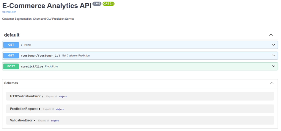
A Living System: The FastAPI Implementation
A model in a notebook is just a report. A model in an API is a product.
I wrapped the entire prediction logic in FastAPI.
• Cold Start Optimization: Models are loaded into memory (artifacts/) only once when the app starts, not for every request.
• Live Prediction Endpoint: /predict/live accepts raw metrics and calculates the segment, churn probability, and CLV instantly.
# src/api.py

@app.post("/predict/live")
def predict_live(req: PredictionRequest):
    # ... (Loading artifacts)

    # Real-time Churn Prediction
    X_churn = pd.DataFrame([[req.frequency, req.monetary, ...]])
    churn_prob = artifacts['churn_model'].predict_proba(X_churn)[0, 1]

    return {
        "churn_probability": float(churn_prob),
        "risk_status": "HIGH" if churn_prob > 0.7 else "Low"
    }
Conclusion: What I Learned & The Road Ahead
This project was more than just fitting a RandomForest to a dataset; it was about understanding the lifecycle of a data product. I learned that the “Modeling” part is only about 20% of the work. The real engineering challenge lies in constructing a clean data pipeline, handling messy real-world edge cases (like Returns), and architecting the code so it doesn’t turn into a “spaghetti script.”
While I am wrapping up this specific project here, I think understanding where it could go next is just as important as building it. If this system were to move into a production environment, in my opinion the logical next steps would be:
• Containerization: Dockerizing the API to ensure it runs consistently across different environments (Dev/Test/Prod).
• Orchestration: Moving the DataIngestion script from a manual run to a scheduled job using Apache Airflow, so the model retrains itself weekly/daily with fresh data.
• Monitoring: Integrating tools like MLflow to track model drift over time (e.g., does the definition of a “VIP” customer change next year?).
For now & for me this repository stands as a solid proof-of-concept for an end-to-end ML workflow. You can find the full source code on my GitHub
Thanks for reading! If you have questions about anything please contact me!
Comments